Categorical Treatments

Use this guide when treatment is categorical, such as control, placebo, and treated.

NoteWhen To Use This Guide

Start here if the treatment is a label rather than a numeric dose. Each distinct observed treatment level is treated as a valid intervention level at prediction time.

Categorical treatments are usually easier to work with than continuous treatments because there is a finite number of treatment levels to predict for. Therefore, some estimators that handle hardest use cases (e.g. continuous treatments) are also able to handle categorical treatments.

To verify available estimators, we can use:

from skcausal.utils.lookup import all_causal_average_response_estimators

all_causal_average_response_estimators(
    as_dataframe=True,
    filter_tags={"capability:t_type": "categorical"},
    return_tags=["capability:t_type"],
)

	name	object	capability:t_type
0	CategoricalDirectMethod	<class 'skcausal.causal_estimators.categorical...	[categorical]
1	CategoricalDoublyRobust	<class 'skcausal.causal_estimators.categorical...	[categorical]
2	CategoricalInversePropensityWeighting	<class 'skcausal.causal_estimators.categorical...	[categorical]
3	DirectNoCovariates	<class 'skcausal.causal_estimators.ignore_cova...	[continuous, categorical]
4	DirectRegressor	<class 'skcausal.causal_estimators.direct_meth...	[continuous, categorical]
5	DoublyRobustPseudoOutcome	<class 'skcausal.causal_estimators.pseudo_outc...	[continuous, categorical]
6	GPS	<class 'skcausal.causal_estimators.gps.GPS'>	[continuous, categorical]
7	Pipeline	<class 'skcausal.causal_estimators.pipeline.Pi...	[continuous, categorical]

We should always give preference doubly robust. But we will see below how to use each of these and how they compare to each other and to the truth on a synthetic dataset.

This example has three levels — "control", "placebo", and "treated" — with known true effects we can verify against.

Step 1: Import dependencies

import numpy as np
import polars as pl
import matplotlib.pyplot as plt

from sklearn.linear_model import LinearRegression, LogisticRegression

from skcausal.causal_estimators import (
    CategoricalDirectMethod,
    CategoricalDoublyRobust,
    CategoricalInversePropensityWeighting,
)
from skcausal.datasets import ExampleCategorical
from skcausal.density.sklearn import SklearnCategoricalDensity
from skcausal.plotting import plot_marginal_curves, use_theme

use_theme()

Step 2: Load a confounded categorical dataset

dataset = ExampleCategorical(n=500, random_state=0)
X, t, y = dataset.load()

pl.concat([X.head(5), t.head(5), y.head(5)], how="horizontal")

shape: (5, 4)

x0	x1	treatment	y
f64	f64	cat	f64
0.12573	1.292893	"control"	0.341335
-0.132105	0.453671	"control"	-0.223364
0.640423	-1.69016	"treated"	1.470218
0.1049	-0.728195	"control"	0.026162
-0.535669	1.232303	"placebo"	-1.09215

The table has two observed covariates, one categorical treatment column, and one outcome column. This is observational data: treatment assignment depends on the covariates, so the raw group means are confounded.

NoteOptional: Exact Data-Generating Process

2a. Create covariates

The dataset samples two observed confounders:

\[ x_0, x_1 \overset{iid}{\sim} \mathcal{N}(0, 1) \]

Both x0 and x1 influence who receives which treatment and what outcome they have — the definition of a confounding variable.

2b. Assign treatments — with confounding

Treatment is assigned by thresholding a linear score that depends on x0 and x1:

\[ s = x_0 - 0.5x_1 + \varepsilon_t, \quad \varepsilon_t \sim \mathcal{N}(0, 0.4^2) \]

\[ T = \begin{cases} \operatorname{treated}, & s > 0.6 \\ \operatorname{placebo}, & s < -0.6 \\ \operatorname{control}, & \text{otherwise} \end{cases} \]

2c. Average response at each treatment level

Using the notation from the methodology page, the true average response function is:

\[ \mu(\text{control}) = 0.8\,\mathbb{E}[x_0] + 0.0, \quad \mu(\text{placebo}) = 0.8\,\mathbb{E}[x_0] - 0.5, \quad \mu(\text{treated}) = 0.8\,\mathbb{E}[x_0] + 1.2 \]

2d. Generate observed outcomes

For each individual unit, the observed outcome is:

\[ Y = 0.8x_0 + \begin{cases} 0.0, & T = \text{control} \\ -0.5, & T = \text{placebo} \\ 1.2, & T = \text{treated} \end{cases} + \varepsilon_y, \quad \varepsilon_y \sim \mathcal{N}(0, 0.2^2) \]

This exact data-generating process is implemented in ExampleCategorical.

The outcome is a linear function of x0 plus the treatment constant plus noise. Notice that x0 drives both treatment assignment (step 2b) and the outcome — this is the confounding the estimators must remove.

Step 3: Define treatment levels

levels = (
    pl.DataFrame({"treatment": ["control", "placebo", "treated"]})
    .with_columns(pl.col("treatment").cast(pl.Categorical))
)

We create the intervention table explicitly here so the three treatment levels being evaluated are visible in the tutorial.

predict accepts the requested treatment table as its first argument and returns one average response per row in levels, averaging over the covariate sample stored during fit.

Step 4: Compute the truth

Because this is a synthetic dataset, we can compute the true average potential outcome exactly from the dataset’s closed-form response function. In the notation from the methodology page, truth_curve contains the three values of \(\mu(t)\) corresponding to the rows in levels.

truth_curve = np.asarray(dataset.predict(X, levels), dtype=float).reshape(-1)
truth = levels.with_columns(pl.Series("truth", truth_curve))

Step 5: Fit the estimators

Direct method

CategoricalDirectMethod fits a regression model for \(E[Y \mid X, T]\) and averages predictions at each treatment level. It relies entirely on the outcome model — no propensity model is needed or fitted:

direct = CategoricalDirectMethod(outcome_regressor=LinearRegression())
direct.fit(X, t, y)

CategoricalDirectMethod(outcome_regressor=LinearRegression())

Please rerun this cell to show the HTML repr or trust the notebook.

direct_curve = direct.predict(t=levels)

This is the fastest estimator to set up and a reliable baseline when the outcome model is well specified. On this dataset, where the outcome is a linear function of x0, a LinearRegression should recover the true effects closely.

Inverse propensity weighting

CategoricalInversePropensityWeighting uses inverse-probability-style correction terms derived from \(P(T = j \mid X)\). With the default target_density_kind="stabilized" used here, the effective correction scale is \(P(T=j) / P(T=j \mid X)\) rather than a raw \(1 / P(T=j \mid X)\) weight. It requires a propensity model:

density_estimator = SklearnCategoricalDensity(LogisticRegression(max_iter=1000))

ipw = CategoricalInversePropensityWeighting(density_estimator=density_estimator)
ipw.fit(X, t, y)

CategoricalInversePropensityWeighting(density_estimator=SklearnCategoricalDensity(classifier=LogisticRegression(max_iter=1000)))

Please rerun this cell to show the HTML repr or trust the notebook.

ipw_curve = ipw.predict(t=levels)

Doubly robust

CategoricalDoublyRobust combines the outcome model and the propensity model. A residual correction from the treatment model adjusts the direct estimate; under the identification conditions above, the estimator is designed to remain consistent if either nuisance model is correctly specified:

dr = CategoricalDoublyRobust(
    density_estimator=density_estimator,
    outcome_regressor=LinearRegression(),
)
dr.fit(X, t, y)

CategoricalDoublyRobust(density_estimator=SklearnCategoricalDensity(classifier=LogisticRegression(max_iter=1000)),
                        outcome_regressor=LinearRegression())

Please rerun this cell to show the HTML repr or trust the notebook.

dr_curve = dr.predict(t=levels)

Tip

Start with doubly robust. Use direct and IPW as sanity checks — if all three land far apart, revisit your nuisance models.

Step 6: Compare to the truth

observed_means = (
    levels.join(
        t.with_columns(y["y"])
        .group_by("treatment")
        .agg(pl.col("y").mean().alias("observed")),
        on="treatment",
        how="left",
    )
)

comparison = (
    observed_means
    .with_columns(
        pl.Series("truth", truth_curve.flatten()),
        pl.Series("direct", direct_curve.flatten()),
        pl.Series("ipw", ipw_curve.flatten()),
        pl.Series("dr", dr_curve.flatten()),
    )
)

comparison

shape: (3, 6)

treatment	observed	truth	direct	ipw	dr
cat	f64	f64	f64	f64	f64
"control"	-0.062448	-0.021512	-0.019108	0.036039	-0.031023
"placebo"	-1.320864	-0.521512	-0.508075	-0.665805	-0.529064
"treated"	1.930502	1.178488	1.149935	0.92153	1.151918

Each row is the estimated average potential outcome under one treatment level. Values close to truth indicate a well-calibrated estimator.

fig, ax = plt.subplots(figsize=(9, 4.5))
plot_marginal_curves(
    levels,
    {
        "Observed": comparison["observed"].to_numpy(),
        "Truth": comparison["truth"].to_numpy(),
        "Direct": comparison["direct"].to_numpy(),
        "IPW": comparison["ipw"].to_numpy(),
        "Doubly robust": comparison["dr"].to_numpy(),
    },
    ax=ax,
)
ax.set_ylabel("Average outcome")
ax.set_title("Observed means vs categorical-treatment estimates")
ax.legend(ncols=3)
plt.show()

The Observed bars are the naive means within each treatment group. Their mismatch with Truth is the confounding signal; the estimator bars show how much of that bias each method removes.

Tip

The average treatment effect of switching from one level to another is simply the difference between the corresponding rows. For example, subtracting the "control" row from the "treated" row gives the average effect of the intervention.

What to try next

If your treatment is numeric and you want a dose-response curve instead, continue to the continuous treatments guide.

NoteOptional: Benchmark the estimators that also handle continuous treatments

The package also exposes general-purpose estimators that can work with categorical treatments here and with continuous treatments in other workflows: DirectRegressor, DoublyRobustPseudoOutcome, and GPS.

Below, we benchmark those estimators on this categorical dataset to show how they compare to the categorical-specific estimators above.

from sklearn.compose import ColumnTransformer, make_column_selector
from sklearn.neighbors import KernelDensity
from sklearn.pipeline import make_pipeline
from sklearn.preprocessing import OneHotEncoder, PolynomialFeatures, SplineTransformer

from skcausal.causal_estimators import (
    DirectNoCovariates,
    DirectRegressor,
    DoublyRobustPseudoOutcome,
    GPS,
)
from skcausal.density.stabilized_from_conditional import (
    KernelMarginalAndConditional,
)


def make_linear_pipeline():
    preprocessor = ColumnTransformer(
        transformers=[
            (
                "encode_categorical",
                OneHotEncoder(
                    drop="first",
                    handle_unknown="ignore",
                    sparse_output=False,
                ),
                make_column_selector(dtype_include=["category", "object", "string"]),
            )
        ],
        remainder="passthrough",
        verbose_feature_names_out=False,
    )
    return make_pipeline(preprocessor, LinearRegression())


def make_gps_outcome_pipeline():
    preprocessor = ColumnTransformer(
        transformers=[
            (
                "expand_gps",
                SplineTransformer(
                    n_knots=5,
                    degree=3,
                    include_bias=False,
                ),
                ["gps"],
            ),
            (
                "encode_categorical",
                OneHotEncoder(
                    drop="first",
                    handle_unknown="ignore",
                    sparse_output=False,
                ),
                make_column_selector(dtype_include=["category", "object", "string"]),
            ),
        ],
        remainder="drop",
        verbose_feature_names_out=False,
    )
    return make_pipeline(
        preprocessor,
        PolynomialFeatures(degree=2, include_bias=False),
        LinearRegression(),
    )


continuous_capable_results = {
    "Truth": truth_curve,
    "DirectNoCovariates": np.asarray(
        DirectNoCovariates(outcome_regressor=make_linear_pipeline())
        .fit(X, t, y)
        .predict(t=levels),
        dtype=float,
    ).reshape(-1),
    "DirectRegressor": np.asarray(
        DirectRegressor(outcome_regressor=make_linear_pipeline())
        .fit(X, t, y)
        .predict(t=levels),
        dtype=float,
    ).reshape(-1),
    "DoublyRobustPseudoOutcome": np.asarray(
        DoublyRobustPseudoOutcome(
            density_estimator=KernelMarginalAndConditional(
                conditional_density_estimator=SklearnCategoricalDensity(
                    LogisticRegression(max_iter=1000)
                ),
                kernel=KernelDensity(bandwidth=0.5),
            ),
            outcome_regressor=make_linear_pipeline(),
            pseudo_outcome_regressor=make_linear_pipeline(),
            random_state=0,
        )
        .fit(X, t, y)
        .predict(t=levels),
        dtype=float,
    ).reshape(-1),
    "GPS": np.asarray(
        GPS(
            density_regressor=SklearnCategoricalDensity(
                LogisticRegression(max_iter=1000)
            ),
            outcome_regressor=make_gps_outcome_pipeline(),
            cv=2,
            random_state=0,
        )
        .fit(X, t, y)
        .predict(t=levels),
        dtype=float,
    ).reshape(-1),
}

continuous_capable_benchmark = levels.with_columns(
    *[
        pl.Series(name, values)
        for name, values in continuous_capable_results.items()
    ]
)

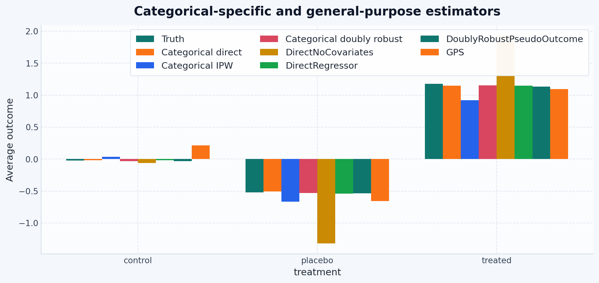
all_estimator_plot_results = {
    "Truth": truth_curve,
    "Categorical direct": direct_curve,
    "Categorical IPW": ipw_curve,
    "Categorical doubly robust": dr_curve,
    "DirectNoCovariates": continuous_capable_results["DirectNoCovariates"],
    "DirectRegressor": continuous_capable_results["DirectRegressor"],
    "DoublyRobustPseudoOutcome": continuous_capable_results[
        "DoublyRobustPseudoOutcome"
    ],
    "GPS": continuous_capable_results["GPS"],
}

continuous_capable_benchmark

shape: (3, 6)

treatment	Truth	DirectNoCovariates	DirectRegressor	DoublyRobustPseudoOutcome	GPS
cat	f64	f64	f64	f64	f64
"control"	-0.021512	-0.062448	-0.016536	-0.030629	0.21502
"placebo"	-0.521512	-1.320864	-0.540517	-0.53553	-0.654686
"treated"	1.178488	1.930502	1.14782	1.132354	1.094306

These estimators trade specialization for a broader treatment interface. On a simple categorical benchmark like this one, that broader interface is convenient for comparing workflows across treatment types, but the fit can differ noticeably from the categorical-specific estimators above. The final plot overlays both families so you can compare everything on the same treatment grid.

fig, ax = plt.subplots(figsize=(12, 5))
plot_marginal_curves(
    levels,
    all_estimator_plot_results,
    ax=ax,
)
ax.set_ylabel("Average outcome")
ax.set_title("Categorical-specific and general-purpose estimators")
ax.legend(ncols=3)
plt.show()

table_comparison = pl.DataFrame({k : np.sqrt(np.mean((v.flatten() - all_estimator_plot_results["Truth"].flatten())**2)) for k,v in all_estimator_plot_results.items() if k != "Truth"}).transpose(include_header=True).rename({"column_0": "RMSE"})
table_comparison = table_comparison.sort("RMSE")
table_comparison

shape: (7, 2)

column	RMSE
str	f64
"Categorical doubly robust"	0.016867
"Categorical direct"	0.018272
"DirectRegressor"	0.021028
"DoublyRobustPseudoOutcome"	0.028331
"GPS"	0.164083
"Categorical IPW"	0.173359
"DirectNoCovariates"	0.634078