Multidimensional Treatments

Use this guide when treatment is stored in more than one column, such as a numeric dose together with a categorical regime.

NoteWhen To Use This Guide

Start here if your treatment table has multiple columns and you want one end-to-end example that stays close to the production API.

What we’re estimating

With multiple treatment coordinates, the target is an Average Response Surface rather than a single curve:

\[ \mu(t_1, \ldots, t_k) = \mathbb{E}_P[Y^*(t_1, \ldots, t_k)] \]

In this example the treatment table has two columns:

  • t_0: one continuous dose
  • t_0_bin: one categorical regime label

So the estimand is

\[ \mu(t, c) = \mathbb{E}_P[Y^*(t, c)] \]

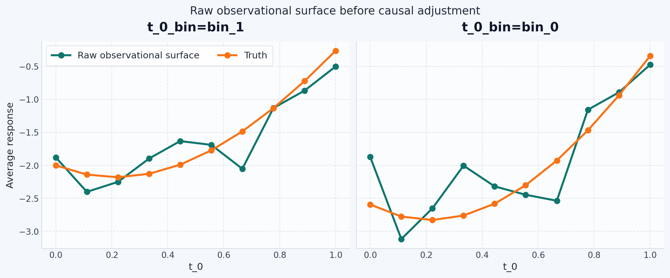
The output is one average response per requested row of a treatment grid. Here we will visualize that surface as one dose-response line per categorical level.

Tip

Think in terms of a treatment table, not a special-case estimator API:

  • fit(X, t, y) takes covariates X, a multi-column treatment table t, and outcomes y
  • grid is another treatment table with the same columns and compatible dtypes
  • predict(t=grid) returns one estimated average response per row in grid

This page compares four estimators that accept the same mixed treatment table:

Estimator Role in this tutorial
DirectNoCovariates Observational baseline: regress Y on the treatment table only
DirectRegressor Outcome regression: model E[Y | X, T] and average over X
GPS Score-adjustment method: add a stabilized treatment score to the outcome model features
DoublyRobustPseudoOutcome Outcome regression plus score correction, followed by a final smoother over treatment
Note

All causal interpretations below assume consistency, no unmeasured confounding after conditioning on X, and overlap across the treatment combinations you want to evaluate.

Step 1: Import dependencies

Code
import numpy as np
import polars as pl
import matplotlib.pyplot as plt

from sklearn.compose import ColumnTransformer
from sklearn.ensemble import RandomForestClassifier, RandomForestRegressor
from sklearn.linear_model import LinearRegression
from sklearn.pipeline import Pipeline
from sklearn.preprocessing import OneHotEncoder, PolynomialFeatures, SplineTransformer

from skcausal.causal_estimators import (
    DirectNoCovariates,
    DirectRegressor,
    DoublyRobustPseudoOutcome,
    GPS,
)
from skcausal.datasets import Synthetic2MultidimDataset
from skcausal.density.permutation_weighting import PermutationWeighting
from skcausal.plotting import plot_joint_curves, use_theme
from skcausal.utils.lookup import (
    all_causal_average_response_estimators,
    all_density_estimators,
)
from skcausal.utils.treatment_grid import make_cartesian_treatment_grid

use_theme()

Step 2: Load a confounded mixed-treatment dataset

Code
dataset = Synthetic2MultidimDataset(
    n=2000,
    n_features=5,
    n_categorical_treatments=2,
    mutual_info=0.7,
    categorical_effect_scale=1.0,
    random_state=0,
)
X, t, y = dataset.load()

X = X.rename({column: f"x{index}" for index, column in enumerate(X.columns)})
continuous_col, categorical_col = t.columns
y = y.rename({y.columns[0]: "y"})

pl.concat([X.head(5), t.head(5), y.head(5)], how="horizontal")
shape: (5, 8)
x0 x1 x2 x3 x4 t_0 t_0_bin y
f64 f64 f64 f64 f64 f64 cat f64
0.361595 1.304 0.947081 -0.703735 -1.265421 0.69931 "bin_1" -1.216821
-0.623274 0.041326 -2.325031 -0.218792 -1.245911 0.350571 "bin_0" -2.704428
-0.732267 -0.544259 -0.3163 0.411631 1.042513 0.3322 "bin_0" -1.50206
-0.128535 1.366463 -0.665195 0.35151 0.90347 0.391606 "bin_1" -1.141317
0.094012 -0.743499 -0.921725 -0.457726 0.220195 0.406004 "bin_0" -2.443491

The table has five observed covariates, one continuous treatment column, one categorical treatment column, and one outcome column.

Synthetic2MultidimDataset starts from the confounded continuous-treatment benchmark SyntheticDataset2, then adds a categorical treatment coordinate by binning the continuous treatment into n_categorical_treatments levels.

The parameter mutual_info=0.7 weakens the link between the two treatment coordinates without removing it completely, and categorical_effect_scale=0.2 makes the categorical coordinate change the response surface directly.

This gives a benchmark where:

  • the continuous dose matters
  • the categorical label matters
  • treatment assignment is still confounded through X
Important

DirectNoCovariates accepts the mixed treatment table, but it does not adjust for confounding. In this dataset, any method that ignores X is still observational.

Step 3: Define practical model builders

The nuisance models below use the same expressive forest defaults. The only deliberate exception is the final doubly robust smoother, which uses a spline basis over the continuous treatment coordinate and a linear regressor over the expanded treatment features.

Code
def make_forest_mixed_treatment_regressor(categorical_column):
    return Pipeline(
        [
            (
                "encode_categorical_treatment",
                ColumnTransformer(
                    [
                        (
                            "categorical_treatment",
                            OneHotEncoder(handle_unknown="ignore", sparse_output=False),
                            [categorical_column],
                        )
                    ],
                    remainder="passthrough",
                    verbose_feature_names_out=False,
                ),
            ),
            (
                "regressor",
                RandomForestRegressor(
                    n_estimators=50,
                    min_samples_leaf=10,
                    random_state=0,
                    n_jobs=-1,
                ),
            ),
        ]
    )
Code
def make_forest_permutation_weighting():
    return PermutationWeighting(
        classifier=RandomForestClassifier(
            n_estimators=50,
            min_samples_leaf=10,
            random_state=0,
            n_jobs=-1,
        ),
        max_trials=50,
        random_state=0,
    )
Code
def make_spline_mixed_treatment_regressor(continuous_column, categorical_column):
    return Pipeline(
        [
            (
                "expand_mixed_treatment",
                ColumnTransformer(
                    [
                        (
                            "expand_continuous_treatment",
                            SplineTransformer(
                                n_knots=8,
                                degree=3,
                                include_bias=False,
                            ),
                            [continuous_column],
                        ),
                        (
                            "encode_categorical_treatment",
                            OneHotEncoder(
                                drop="first",
                                handle_unknown="ignore",
                                sparse_output=False,
                            ),
                            [categorical_column],
                        ),
                    ],
                    remainder="drop",
                    verbose_feature_names_out=False,
                ),
            ),
            (
                "interaction_terms",
                PolynomialFeatures(
                    degree=2,
                    interaction_only=True,
                    include_bias=False,
                ),
            ),
            ("regressor", LinearRegression()),
        ]
    )
Code
def mean_absolute_error(left, right):
    return float(np.mean(np.abs(np.asarray(left) - np.asarray(right))))

Step 4: Build the intervention grid

Code
grid = make_cartesian_treatment_grid(
    t,
    n_continuous_points=10,
)

grid.head(8)
shape: (8, 2)
t_0 t_0_bin
f64 cat
3.3844e-7 "bin_1"
3.3844e-7 "bin_0"
0.111111 "bin_1"
0.111111 "bin_0"
0.222222 "bin_1"
0.222222 "bin_0"
0.333333 "bin_1"
0.333333 "bin_0"

make_cartesian_treatment_grid replaces each continuous treatment column with evenly spaced points, keeps the observed categorical levels, and returns the Cartesian product. In this example that means 10 dose values times 2 categorical levels.

Note

The prediction contract is unchanged from the single-treatment guides: pass a treatment table to predict, and get back one average response per row of that table.

Step 5: Compute the truth

truth_curve = dataset.predict(X, grid).flatten()
truth = grid.with_columns(pl.Series("truth", truth_curve))

Because this is a synthetic dataset, we can evaluate the true average potential outcome surface exactly for every row in grid. That makes the rest of the tutorial a benchmarking exercise, not just an API example.

Step 6: Inspect the raw observational surface

Code
naive = DirectNoCovariates(
    outcome_regressor=make_forest_mixed_treatment_regressor(categorical_col)
)
naive.fit(X, t, y)
naive_curve = naive.predict(t=grid).flatten()
fig, axes = plt.subplots(
    1,
    len(dataset.levels_),
    figsize=(11, 4.5),
    sharey=True,
    constrained_layout=True,
)
axes = np.atleast_1d(axes)
plot_joint_curves(
    grid,
    {
        "Raw observational surface": naive_curve,
        "Truth": truth_curve,
    },
    ax=axes,
    separate_axes_by_group=True,
)
fig.suptitle("Raw observational surface before causal adjustment")
axes[0].legend(ncols=2)
plt.show()

DirectNoCovariates is a useful observational baseline, but it is not a causal estimate. The model ignores X, so even after splitting by t_0_bin, the continuous dose remains confounded by the covariates.

Step 7: Fit DirectRegressor

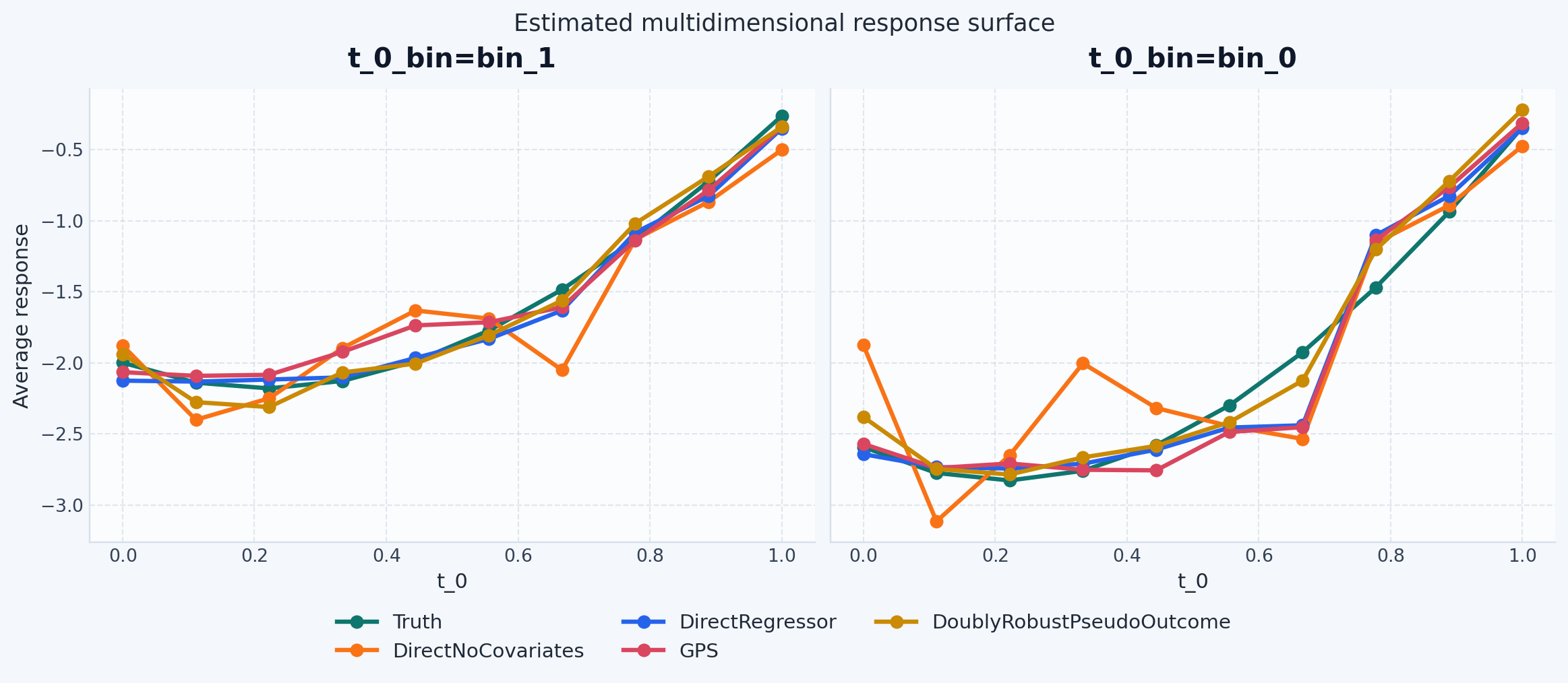
DirectRegressor uses the same mixed-treatment outcome model, but now the model sees both X and the treatment table. Prediction averages over the observed covariate sample at each requested treatment row.

direct = DirectRegressor(
    outcome_regressor=make_forest_mixed_treatment_regressor(categorical_col)
)
direct.fit(X, t, y)
direct_curve = direct.predict(t=grid).flatten()

Step 8: Fit GPS

GPS augments the outcome model with a treatment score computed from predict_density(X, t). In this example that score comes from PermutationWeighting, which returns a stabilized density-ratio-style quantity. So this is best read as a score-adjustment example, not as a parametric conditional-density example.

gps = GPS(
    density_regressor=make_forest_permutation_weighting(),
    outcome_regressor=make_forest_mixed_treatment_regressor(categorical_col),
    cv=2,
    max_samples_predict=500,
    random_state=0,
)
gps.fit(X, t, y)
gps_curve = gps.predict(t=grid).flatten()

Step 9: Fit DoublyRobustPseudoOutcome

DoublyRobustPseudoOutcome uses the same forest outcome model and the same stabilized score model, then smooths the pseudo-outcomes over treatment with a spline basis over the continuous coordinate and encoded indicators for the categorical coordinate.

dr = DoublyRobustPseudoOutcome(
    density_estimator=make_forest_permutation_weighting(),
    outcome_regressor=make_forest_mixed_treatment_regressor(categorical_col),
    pseudo_outcome_regressor=make_spline_mixed_treatment_regressor(
        continuous_col,
        categorical_col,
    ),
    cv=2,
    cross_fit=True,
    random_state=0,
)
dr.fit(X, t, y)
dr_curve = dr.predict(t=grid).flatten()

Step 10: Compare estimates

comparison = grid.with_columns(
    pl.Series("truth", truth_curve),
    pl.Series("DirectNoCovariates", naive_curve),
    pl.Series("DirectRegressor", direct_curve),
    pl.Series("GPS", gps_curve),
    pl.Series("DoublyRobustPseudoOutcome", dr_curve),
)

comparison.head(8)
shape: (8, 7)
t_0 t_0_bin truth DirectNoCovariates DirectRegressor GPS DoublyRobustPseudoOutcome
f64 cat f64 f64 f64 f64 f64
3.3844e-7 "bin_1" -1.999153 -1.878706 -2.125528 -2.065738 -1.938303
3.3844e-7 "bin_0" -2.593063 -1.872583 -2.642717 -2.570411 -2.380102
0.111111 "bin_1" -2.139635 -2.400981 -2.132084 -2.091885 -2.276765
0.111111 "bin_0" -2.77528 -3.115715 -2.733742 -2.740464 -2.746407
0.222222 "bin_1" -2.180113 -2.249773 -2.117787 -2.084515 -2.311381
0.222222 "bin_0" -2.827783 -2.650613 -2.744197 -2.708539 -2.786131
0.333333 "bin_1" -2.12773 -1.89681 -2.102549 -1.923527 -2.06814
0.333333 "bin_0" -2.759838 -2.003625 -2.710003 -2.752775 -2.665716
Code
fig, axes = plt.subplots(
    1,
    len(dataset.levels_),
    figsize=(12, 5.2),
    sharey=True,
    constrained_layout=True,
)
axes = np.atleast_1d(axes)
plot_joint_curves(
    grid,
    {
        "Truth": truth_curve,
        "DirectNoCovariates": naive_curve,
        "DirectRegressor": direct_curve,
        "GPS": gps_curve,
        "DoublyRobustPseudoOutcome": dr_curve,
    },
    ax=axes,
    separate_axes_by_group=True,
)
handles, labels = axes[0].get_legend_handles_labels()
axis_legend = axes[0].get_legend()
if axis_legend is not None:
    axis_legend.remove()
fig.suptitle("Estimated multidimensional response surface")
fig.legend(
    handles,
    labels,
    loc="outside lower center",
    ncols=3,
    frameon=False,
)
plt.show()

pl.DataFrame(
    {
        "estimator": [
            "DirectNoCovariates",
            "DirectRegressor",
            "GPS",
            "DoublyRobustPseudoOutcome",
        ],
        "mean_absolute_error": [
            mean_absolute_error(naive_curve, truth_curve),
            mean_absolute_error(direct_curve, truth_curve),
            mean_absolute_error(gps_curve, truth_curve),
            mean_absolute_error(dr_curve, truth_curve),
        ],
    }
).sort("mean_absolute_error")
shape: (4, 2)
estimator mean_absolute_error
str f64
"DoublyRobustPseudoOutcome" 0.10216
"DirectRegressor" 0.105087
"GPS" 0.130103
"DirectNoCovariates" 0.278844

Treat the MAE table as a compact summary, not the whole story. The faceted plot is still the best place to see whether an estimator misses one categorical level or only part of the dose range.

Note

With shared forest nuisance models in place, the remaining differences are more about estimator structure and stochastic variation than about an obviously underpowered outcome or score model. The doubly robust estimator still uses a different final smoother by design.

Optional: Verify discovered support with lookup

The main tutorial above uses four estimators because those are the current average-response estimators tagged as supporting both multidimensional treatments and mixed continuous/categorical treatment types.

estimator_catalog = all_causal_average_response_estimators(
    as_dataframe=True,
    filter_tags={"capability:multidimensional_treatment": True},
    return_tags=["capability:t_type", "capability:multidimensional_treatment"],
)

mixed_treatment_estimators = estimator_catalog[
    estimator_catalog["capability:t_type"].apply(
        lambda values: {"continuous", "categorical"}.issubset(set(values))
    )
][["name", "capability:t_type", "capability:multidimensional_treatment"]].reset_index(
    drop=True
)

mixed_treatment_estimators
name capability:t_type capability:multidimensional_treatment
0 DirectNoCovariates [continuous, categorical] True
1 DirectRegressor [continuous, categorical] True
2 DoublyRobustPseudoOutcome [continuous, categorical] True
3 GPS [continuous, categorical] True
density_catalog = all_density_estimators(
    as_dataframe=True,
    filter_tags={"capability:multidimensional_treatment": True},
    return_tags=["capability:t_type", "capability:multidimensional_treatment"],
)

mixed_treatment_densities = density_catalog[
    (density_catalog["name"] != "Pipeline")
    & density_catalog["capability:t_type"].apply(
        lambda values: {"continuous", "categorical"}.issubset(set(values))
    )
][["name", "capability:t_type", "capability:multidimensional_treatment"]].reset_index(
    drop=True
)

mixed_treatment_densities
name capability:t_type capability:multidimensional_treatment
0 CompositeFactorizedDensityEstimator [continuous, categorical] True
1 NaiveDensityEstimator [continuous, categorical] True
2 PermutationWeighting [continuous, categorical] True